Gallery

Reproducible reaction-profile figures. Each is rebuilt by python goodvibes/examples/gallery/build_gallery.py from compact files in the repository (reaction-profile documents with embedded conformers, and a CSV table); no program output is needed. The inputs, the code of every figure and the commands are in goodvibes/examples/gallery.

Δqh-G with every conformer

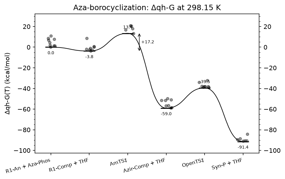
Aza-borocyclization Δqh-G profile with conformers

One computed series at 298.15 K from about 100 Gaussian outputs, transition states labelled above their bar, each conformer drawn around its species’ level, and a barrier annotation.

One profile at four temperatures

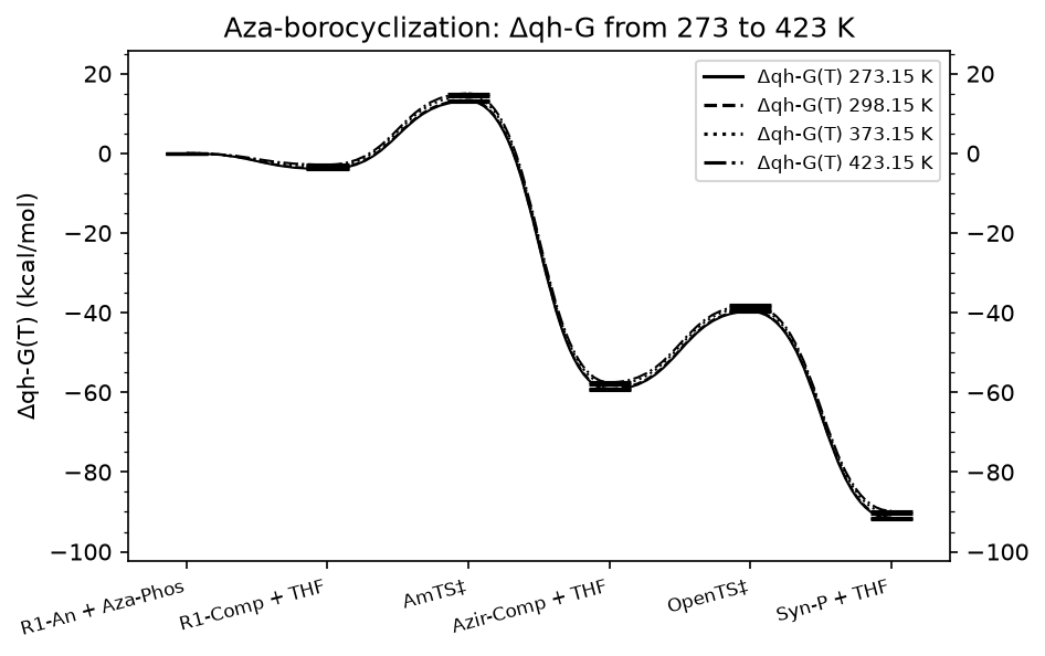
The embedded structures re-evaluated at each temperature without the output files: goodvibes-profile plot goodvibes/examples/profiles/azabor_profile.json --temperatures 273.15,298.15,373.15,423.15 -o scan.png.

ΔE, ΔH and Δqh-G on one axes

ΔE, ΔH and Δqh-G of one profile

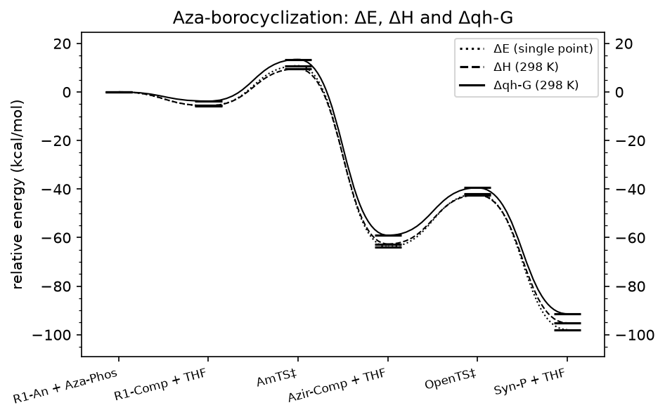
Three quantities of the same structures as three series.

Competing transition states, one panel each

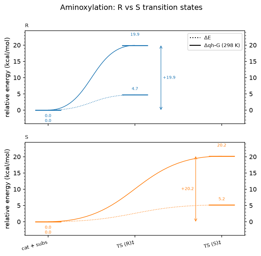
R and S transition states in two panels

Two pathways from one reactant pair (layout: panels), ΔE dotted and Δqh-G solid, barriers marked.

A CSV table of relative energies

A profile drawn from a CSV table

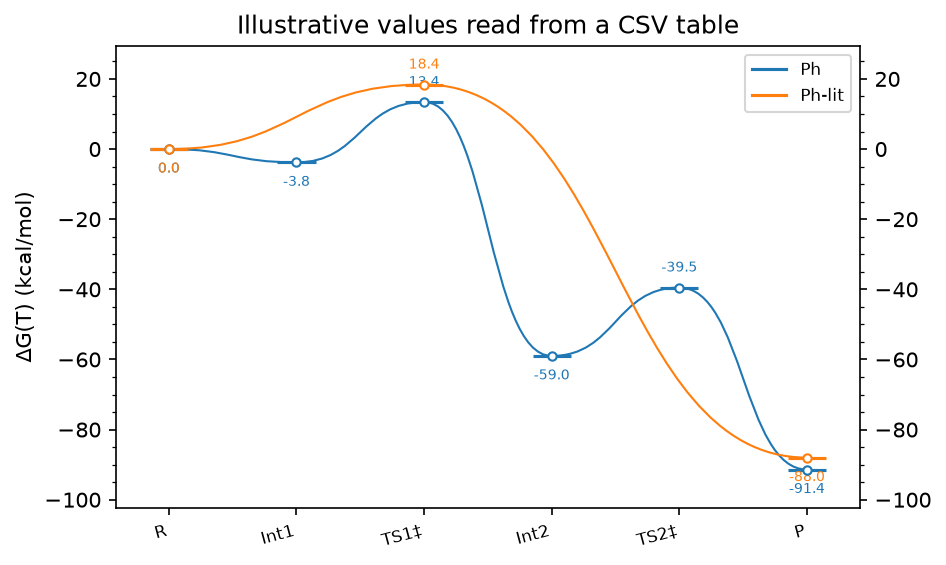
goodvibes-profile plot goodvibes/examples/profiles/levels.csv -o levels.png: a hand-typed table is a profile. The values are illustrative, not from a publication.

Computed and declared values together

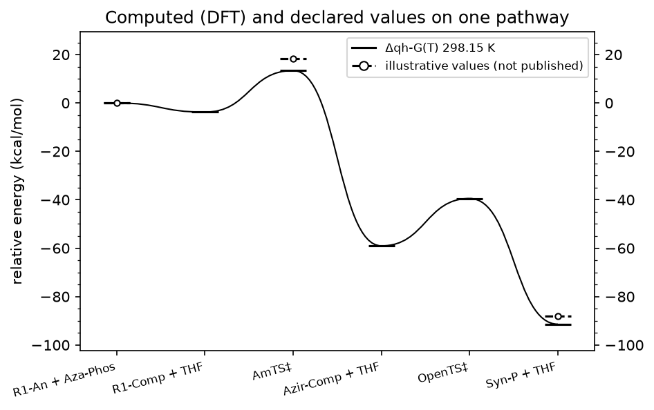
Computed and declared series on one pathway

A declared series (hollow markers; illustrative values) next to the computed Δqh-G on the same points.

A journal-column preset with error bars

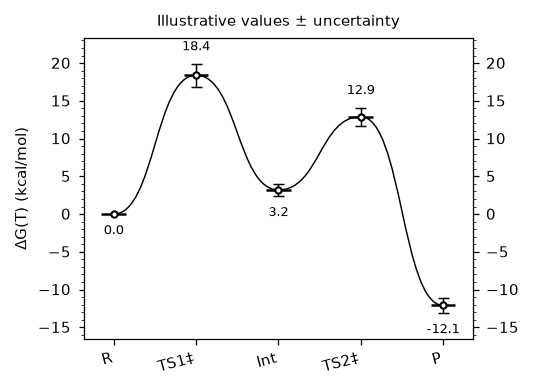
A declared profile with error bars at the single-column preset

minimal.yaml with illustrative ± uncertainties added, drawn at the single-column preset. Saved as SVG, the figure keeps its text editable and embeds the drawn document.

from goodvibes import load_profile

prof = load_profile("goodvibes/examples/profiles/minimal.yaml")
prof.series[0].uncertainty = {"main": {"TS1": 1.5, "Int": 0.8, "TS2": 1.2, "P": 1.0}}
prof.plot(preset="single-column", label_points=True).save("fig.svg", "fig.pdf")

In a document the uncertainties sit under the series as uncertainty:, next to levels:; goodvibes-profile plot profile.yaml -o fig.svg --preset single-column then draws the same figure.